I have just released new versions of two Mathematica packages I have written only today:
Carlson 1.1 (computing Carlson integrals)
![]()
MoleculeViewer 3.0 (molecule visualization)
![]()
The bulk of the work for these two Mathematica packages was already done many months ago, but was greatly hampered by not having a working computer of my own to use. Recently, kind friends (including some readers of this blog) have helped contribute to getting my computer fixed, which enabled me to put the finishing touches to these packages.
Nevertheless, it seems my little netbook is not long for this world, as the technicians at the repair center have advised me that getting it fixed in the future would be even more difficult due to parts availability. Thankfully, I now have backups of my research (all in various stages of completion and rigor) and artwork on another hard disk, so the situation is not like the time this very same computer was saved from the pawn shop.
Additionally, altho my software is and will always remain free for use, the electricity and Internet conection needed for me to do research and experimentation is not. Thus, I have set up a Ko-fi page for people who may want to contribute to letting me do more research, and facilitate the release of my unpublished work. (Perhaps if I get enough help, I might be able to finally work on a 64-bit computer!)
So, for users of previous versions of my packages, please do try out these new releases, and if you can perhaps spare some change, your help would be very much appreciated!
(As always, people with my personal e-mail address can drop a line for more details.)
I owe a lot of what I know to the kindness of the Internet, and I hope I can keep on contributing back.
~ Jan
 of quaternion argument. Working through the derivation resulted in a lovely formula, and I have decided to write this post to put the resulting formula on record.
 (i.e., the quaternion with scalar part
  and vector part
  ) with the complex matrix
 . Using either the Jordan normal form or the Cauchy integral definition of a matrix function (see e.g.
 .
. or
or  , this gives results consistent with formulae based on the quaternionic version of the Euler formula,
 . For functions with branch cuts, however, care is necessary, since the result might not be consistent with the result of a different method.
 and
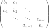
and  in Usmani’s notation. As noted in his papers, they can be generated through a three term recurrence; thus, another way to implement
  matrices built from the diagonal and off-diagonal elements of the tridiagonal matrix, partly because I wanted to demonstrate this method.
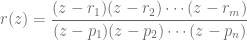
 are the zeroes, and the
  are the poles. Less well-known is the fact that any doubly periodic (i.e., elliptic) function can also be decomposed into its zeroes and poles.
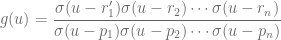
 and
and  are the half-periods, such that their
  has positive imaginary part. Additionally, the quantity
  is defined to be
 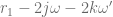 , where
  and
and  are integers chosen such that
  .
.
 roots of the trinomial equation
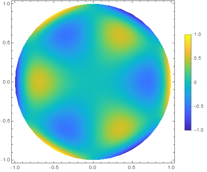
 -function
 . I will post details at another time, and will just mention that Mathematica is not able to come up with a closed-form solution for this DE.
 defined by the relation
  , then
 .
.